?An Unhealthy Commute The following data represent commute times (in minutes) and a score on a well-being survey. Use the results from P

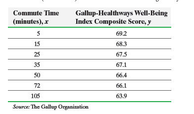
The full step-by-step solution to problem: 11 from chapter: 14.1 was answered by , our top Statistics solution expert on 01/15/18, 03:19PM. The answer to “?An Unhealthy Commute The following data represent commute times (in minutes) and a score on a well-being survey. Use the results from in Section 4.2 to answer the following questions:(a) Treating commute time as the explanatory variable, x, determine the estimates of 0 and 1.(b) Compute the standard error of the estimate, Se.(c) Determine Sb1.(d) A normal probability plot of the residuals indicates it is reasonable to conclude the residuals are normally distributed. Test whether a linear relation exists between commute time and well-being index composite score at the a = 0.05 level of significance.(e) Construct a 95% confidence interval about the slope of the true least-squares regression line.” is broken down into a number of easy to follow steps, and 109 words. Statistics: Informed Decisions Using Data was written by and is associated to the ISBN: 9780134133539. This textbook survival guide was created for the textbook: Statistics: Informed Decisions Using Data, edition: 5. Since the solution to 11 from 14.1 chapter was answered, more than 218 students have viewed the full step-by-step answer. This full solution covers the following key subjects: . This expansive textbook survival guide covers 88 chapters, and 2422 solutions.