The Paris GunsContinued Mathematically, Galileos model in is perfect. But in practice it

Chapter 3, Problem 62

(choose chapter or problem)

The Paris Guns—Continued Mathematically, Galileo’s model in Problem 61 is perfect. But in practice it is only as accurate as the hypotheses upon which it is based. The motion of a real projectile is resisted to some extent by the air, and the stronger this effect, the less realistic are the hypotheses of constant horizontal velocity and constant vertical acceleration, as well as the resulting independence of the projectile’s motion in the x and y directions.

The first successful model of air resistance was formulated by the Dutch scientist Christiaan Huygens (1629–1695) and Isaac Newton (1643–1727). It was based not so much on a detailed mathematical formulation of the underlying physics involved, which was beyond what anyone could manage at the time, but on physical intuition and groundbreaking experimental work. Newton’s version, which is known to this day as Newton’s law of air resistance, states that the resisting force or drag force on an object moving through a resisting medium acts in the direction opposite to the direction of the object’s motion with a magnitude proportional to the density \(\rho\) of the medium, the cross sectional area A of the object taken perpendicular to the direction of motion, and the square of the speed \(\|\mathbf{v}\|\) of the object. In modern vector notation, the drag force is a vector \(f_{D}\) given in terms of the velocity v of the object:

\(f_{D}=-\frac{1}{2} C \rho A\|\mathbf{v}\|^{2} \frac{\mathbf{v}}{\|\mathbf{v}\|}=-\frac{1}{2} C \rho A\|\mathbf{v}\| \mathbf{v}\),

where in the coordinate system of Problem 61 the velocity is the vector \(\mathbf{v}=\langle d x / d t, d y / d t\rangle\). When the force of gravity and this drag force are combined according to Newton’s second law of motion we get:

\(m\left\langle\frac{d^{2} x}{d t^{2}}, \frac{d^{2} y}{d t^{2}}\right\rangle=\langle 0,-m g\rangle+f_{D}\).

The initial-value problem (2) is then modified to read:

\(m \frac{d^{2} x}{d t^{2}}=-\frac{1}{2} C \rho A\left[\sqrt{\left(\frac{d x}{d t}\right)^{2}+\left(\frac{d x}{d t}\right)^{2}}\right] \frac{d x}{d t}\)

\(m \frac{d^{2} y}{d t^{2}}=-m g-\frac{1}{2} C \rho A\left[\sqrt{\left(\frac{d x}{d t}\right)^{2}+\left(\frac{d x}{d t}\right)^{2}}\right] \frac{d y}{d t}\)

where x(0)=0, y(0)=0, \(x^{\prime}(0)=v_{0} \cos \theta\), \(y^{\prime}(0)=v_{0} \sin \theta\).

Huygens seemed to believe that the proportionality of drag force to the square of the speed was universal, but Newton suspected that multiple different physical effects contributed to drag force, not all of which behaved that way. He turned out to be correct. For example, when the speed of an object is low enough compared to the viscosity (internal resistance to flow) of the medium, drag force ends up being approximately proportional to its speed (not the square of its speed), a relationship known as Stokes’ law of air resistance. Even today, there is no quick recipe for predicting the drag force for all objects under all conditions. The modeling of air resistance is complicated and is done in practice by a combination of theoretical and empirical methods. The coefficient C in (3) is called the drag coefficient. It is dimensionless (that is, it is the same no matter what units are used to measure mass, distance, and time) and it can usually be regarded as depending only on the shape of a projectile and not on its size. The drag coefficient is such a convenient index for measuring how much air resistance is felt by a projectile of a given shape that it is now defined in terms of the drag force to be \(2\left\|f_{D}\right\| /\left(\rho A\|\mathbf{v}\|^{2}\right.\)) even when this ratio cannot be regarded as constant. For example, under Stokes’ law of air resistance, C would be proportional to the reciprocal of the speed. Of greater concern to us is the fact that the drag coefficient of a projectile in air increases sharply as its speed approaches the speed of sound (approximately 340 m/s in air), then decreases gradually for even higher speeds, becoming nearly constant again for speeds several times the speed of sound. This was first discovered by the military engineer Benjamin Robins (see Problem 57), whose book Principles of Gunnery is generally regarded as inaugurating the modern age of artillery and of the science of ballistics in general. As guns were used to shoot projectiles further and further with greater and greater initial speeds throughout the eighteenth and nineteenth centuries, the dependence of the drag coefficient on speed took on greater and greater practical importance. Moreover, as these projectiles went higher and higher, the fact that the density of the air decreases with increasing altitude also became important. By World War I, the density of the air as a function of altitude y above sea level in meters was commonly modeled by the function:

\(\rho(y)=1.225 e^{-0.00010361 y} \mathrm{\ kg} / \mathrm{m}^{3}\)

and military engineers were accustomed to incorporating into (3) the dependence of C on velocity and of \(\rho\) on y. But one last major surprise was stumbled upon by German engineers during World War I. Our version of this story is based on the book Paris Kanonen—the Paris Guns (Wilhelmgeschütze) and Project HARP by Gerald V. Bull (Verlag E. S. Mittler & Sohn GmbH, Herford, 1988).

In the fall of 1914, the German Navy charged the Friedrich Krupp engineering firm with designing a system (gun and shells) capable of bombing the English port of Dover from the French coast. This would require firing a shell approximately 37 kilometers, a range some 16 kilometers greater than had ever been achieved before. Krupp was ready for this challenge because it had already succeeded in designing and building shells with innovative shapes that had lower drag coefficients than any pre war shells. The drag coefficient for one of these shells can be well approximated by the following piecewise linear function, where the speed v is in m/s:

\(C(v)=\left\{\begin{array}{lr}0.2, & 0<v<306 \\0.2+(v-306) / 340, & 306 \leq v<374 \\0.4-(v-374) / 3230, & 374 \leq v<1020 \\0.2, & v>1020\end{array}\right.\).

In addition, Krupp’s engineers already had built an experimental gun having a 35.5 cm diameter barrel that could fire 535 kg shells with an initial speed of 940 m/s. They calculated that if they built one of their new low-drag shells with that diameter and mass and used this gun to launch it at a \(43^{\circ}\) angle to the horizontal, the shell should have a range of about 39 km. The shell was built, and a test firing was conducted on October 21, 1914. For the results, we quote a first-hand account by Professor Fritz Rausenberger, managing director of the Krupp firm at the time (from pages 24–25 in Bull’s book):

“After the firing of the first shot, with a top zone propelling charge and at \(43^{\circ}\) elevation, we all waited with anxiety for the spotting report to be telephoned back to us giving the location of the inert shell impact. The anxiety was that normally associated when trying to reach a range never before achieved. But the spotter’s report on impact never came. None of the observers located along the full length of the range had observed impact …

Since no observation posts had been established beyond the 40 km mark, any impact outside of the area would have to be located and reported by local inhabitants using normal telephone communication between the neighbouring farms and villages. Thus it took several hours before the range staff received notification that the shell had impacted in a garden (without causing damage) some 49 km down-range from the battery. This was an unexpectedly favorable result but raised the question of how the range increase of 25% over that predicted using standard exterior ballistic techniques occurred .... After careful study of the method of calculating range, it was clear that in the computations an average, constant air density was used which was larger than the average along the trajectory. The method of calculating trajectory was therefore changed to allow for variation of density along the trajectory. This was done by dividing the atmosphere into 3 km bands from the Earth’s surface upwards. For each band an average air density value was determined and applied over that portion of the trajectory falling in this band. This step-by-step calculation technique was carried out from the muzzle until impact. The resultant calculated trajectory, using the drag coefficient as determined from small calibre firings, matched closely the experimental results from the 21st of October Meppen firing.”

Note that Rausenberger does not tell us what “average, constant” air density was used in the faulty calculation, or how it was determined. Actually, there is a logical problem here in that it is not possible to know how low the air density will become along the path of a trajectory without already knowing how high the trajectory will go. Nevertheless the engineers were confident of their calculations, so it seems likely that they did not regard the air density as a critical parameter when their concern was only to find an approximate range. (After all, they had never shot anything so high before.)

(a) Use a computer algebra system to write a routine that can numerically solve (3) with the piecewise defined C and exponentially decaying r given above and graph the resulting trajectory in the xy-plane. (You may need to rewrite (3) as a first-order system. See Section 6.4.) The area A is that of a circle with the diameter of the shell. Test your routine on the case \(\rho=0\) which was solved analytically in Problem 61.

(b) Suppose that, as Krupp engineers, we use the results of part (c) in Problem 61 to calculate the maximum height M that would have been attained by the test shell had it been launched in a vacuum \((\rho=0)\), then figure that the real test shell might reach about half that height, and finally settle on a “constant, average” value for \(\rho\) of \((\rho(M / 2)+\rho(0)) / 2\). Plot the resulting trajectory, and show that the resulting range is uncannily close to that predicted by the Krupp engineers for the October 14, 1914, test.

(c) Note that the launch angle for this test was not the \(45^{\circ}\) angle that yields maximum range in a vacuum, but a smaller \(43^{\circ}\) angle. Does this smaller launch angle lead to greater range under the constant air density assumption that you used in part (b)? To the nearest degree, what launch angle yields maximum range according to this model?

(d) Now plot the trajectory of the test shell using the proper exponentially decaying \(\rho\). What happens? (In evaluating the results, it should make you feel better that we are not pretending to take everything into account in this model. For example, a missile moving at an angle relative to its axis of symmetry can experience a substantial lift force of the same sort that makes airplanes fly. Our model does not account for the possibility of lift, the curvature and rotation of the Earth, or numerous other effects.)

Rausenberger notes that once his engineers realized how important the exponentially decaying \(\rho\) was in calculating range, they did a series of calculations and found that the maximum range for their test would actually have been achieved with a launch angle of \(50^{\circ}\) to \(55^{\circ}\).  In hindsight, they realized that this was because a larger launch angle would result in the shell traveling higher and therefore in less dense air.

(e) Check this by plotting the trajectory of the test shell with exponentially decaying \(\rho\) every two degrees from \(43^{\circ}\) to \(55^{\circ}\) . What do you find?

After these surprising results, engineers at Krupp became interested in the challenge of attaining even larger ranges. The only way they could think of to talk the German High Command into committing to the trouble and expense of pursuing this goal was to sell them on the possibility of bombing Paris from behind the German front line, which would require a range of some 120 km. The German High Command quickly approved this idea, and after several years of work Krupp produced what are now known as the Paris Guns. These guns were designed to launch a 106 kg shell having a diameter of 216 mm with an initial velocity of 1646 m/s. At a \(50^{\circ}\) launch angle, such a shell was predicted to travel over 120 km.

                                   

(f) Simulate the trajectory of a shell from a Paris Gun using (2) with exponentially decaying \(\rho\). Evaluate the results keeping in mind the caveats about our modeling noted in part (d). How high does the shell go? Now change the launch angle from \(50^{\circ}\) to \(45^{\circ}\). What happens?

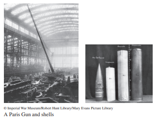
Seven Paris Guns were built, but only three were used. They fired a total of 351 shells towards Paris between March 23 and August 9 of 1918. The damage and casualties that they caused were not tactically significant. They were never intended to be so; there was no control over where the shells would fall in Paris, and the amount of explosive carried by each shell was quite small. Instead, they were intended as a form of intimidation, a “scare tactic.” However, military historians agree that they were not effective in that sense either. Their significance turned out to be more scientific than military. The shells that they launched were the first man-made objects to reach the stratosphere, initiating the space age in the science of ballistics.