In each of Problems 1 through 4: G a. Draw a direction field and sketch a few trajectories. b. Express the general solution of the given system of equations in terms of real-valued functions. c. Describe the behavior of the solutions as t .x_ = _1 4 1 1 _ x
Read moreTable of Contents
1.1
Some Basic Mathematical Models; Direction Fields
1.2
Solutions of Some Differential Equations
1.3
Classification of Differential Equations
2
First-Order Differential Equations
2.1
Linear Differential Equations; Method of Integrating Factors
2.2
Separable Differential Equations
2.3
Modeling with First-Order Differential Equations
2.4
Differences Between Linear and Nonlinear Differential Equations
2.5
Autonomous Differential Equations and Population Dynamics
2.6
Exact Differential Equations and Integrating Factors
2.7
Numerical Approximations: Eulers Method
2.8
The Existence and Uniqueness Theorem
2.9
First-Order Difference Equations
3.1
Homogeneous Differential Equations with Constant Coefficients
3.2
Solutions of Linear Homogeneous Equations; the Wronskian
3.3
Complex Roots of the Characteristic Equation
3.4
Repeated Roots; Reduction of Order
3.5
Nonhomogeneous Equations; Method of Undetermined Coefficients
3.6
Variation of Parameters
3.7
Mechanical and Electrical Vibrations
3.8
Forced Periodic Vibrations
4.1
General Theory of nth Order
4.2
Homogeneous Differential Equations with Constant Coefficients
4.3
The Method of Undetermined Coefficients
4.4
The Method of Variation of Parameters
5.1
Review of Power Series
5.2
Series Solutions Near an Ordinary Point, Part I
5.3
Series Solutions Near an Ordinary Point, Part II
5.4
Euler Equations; Regular Singular Points
5.5
Series Solutions Near a Regular Singular Point, Part I
5.6
Series Solutions Near a Regular Singular Point, Part II
5.7
Bessels Equation
6.1
Definition of the Laplace Transform
6.2
Solution of Initial Value Problems
6.3
Step Functions
6.4
Differential Equations with Discontinuous Forcing Functions
6.5
Impulse Functions
6.6
The Convolution Integral
7.1
Introduction
7.2
Matrices
7.3
Systems of Linear Algebraic Equations; Linear Independence, Eigenvalues, Eigenvectors
7.4
Basic Theory of Systems of First-Order Linear Equations
7.5
Homogeneous Linear Systems with Constant Coefficients
7.6
Complex-Valued Eigenvalues
7.7
Fundamental Matrices
7.8
Repeated Eigenvalues
7.9
Nonhomogeneous Linear Systems
8.1
The Euler or Tangent Line Method
8.2
Improvements on the Euler Method
8.3
The Runge-Kutta Method
8.4
Multistep Methods
8.5
Systems of First-Order Equations
8.6
More on Errors; Stability
9.1
The Phase Plane: Linear Systems
9.2
Autonomous Systems and Stability
9.3
Locally Linear Systems
9.4
Competing Species
9.5
Predator -- Prey Equations
9.6
Liapunovs Second Method
9.7
Periodic Solutions and Limit Cycles
9.8
Chaos and Strange Attractors: The Lorenz Equations
10.1
Two-Point Boundary Value Problems
10.2
Fourier Series
10.3
The Fourier Convergence Theorem
10.4
Even and Odd Functions
10.5
Separation of Variables; Heat Conduction in a Rod
10.6
Other Heat Conduction Problems
10.7
The Wave Equation: Vibrations of an Elastic String
10.8
Laplaces Equation
11.1
The Occurrence of Two-Point Boundary Value Problems
11.2
Sturm-Liouville Boundary Value Problems
11.3
Nonhomogeneous Boundary Value Problems
11.4
Singular Sturm-Liouville Problems
11.5
Further Remarks on the Method of Separation of Variables: A Bessel Series Expansion
11.6
Series of Orthogonal Functions: Mean Convergence
Textbook Solutions for Elementary Differential Equations and Boundary Value Problems
Chapter 7.6 Problem 16
Question
In each of 16 and 17, solve the given system of equations by the method of of Section 7.5. Assume that t > 0.tx_ = _1 1 2 1 _ x 1
Solution
Step 1 of 5
In order to find the eigenvalues we need to calculate for which 
Hence, the eigenvalues of the coefficient matrix are 
Subscribe to view the
full solution
full solution
Title
Elementary Differential Equations and Boundary Value Problems 11
Author
Boyce, Diprima, Meade
ISBN
9781119256007
Solved: In each of 16 and 17, solve the given system of equations by the method of of
Chapter 7.6 textbook questions
-
Chapter 7: Problem 1 Elementary Differential Equations and Boundary Value Problems 11
-
Chapter 7: Problem 2 Elementary Differential Equations and Boundary Value Problems 11
In each of Problems 1 through 4: G a. Draw a direction field and sketch a few trajectories. b. Express the general solution of the given system of equations in terms of real-valued functions. c. Describe the behavior of the solutions as t .x_ = _2 5 1 2 _ x
Read more -
Chapter 7: Problem 3 Elementary Differential Equations and Boundary Value Problems 11
In each of Problems 1 through 4: G a. Draw a direction field and sketch a few trajectories. b. Express the general solution of the given system of equations in terms of real-valued functions. c. Describe the behavior of the solutions as t .x_ = _1 1 5 3 _ x
Read more -
Chapter 7: Problem 4 Elementary Differential Equations and Boundary Value Problems 11
In each of Problems 1 through 4: G a. Draw a direction field and sketch a few trajectories. b. Express the general solution of the given system of equations in terms of real-valued functions. c. Describe the behavior of the solutions as t .x_ = _ 1 2 5 1 _ X
Read more -
Chapter 7: Problem 5 Elementary Differential Equations and Boundary Value Problems 11
In each of Problems 5 and 6, express the general solution of the given system of equations in terms of real-valued functions.x_ = 1 0 0 2 1 2 3 2 1 x
Read more -
Chapter 7: Problem 6 Elementary Differential Equations and Boundary Value Problems 11
In each of Problems 5 and 6, express the general solution of the given system of equations in terms of real-valued functions.x_ = 3 0 2 1 1 0 2 1 0 x
Read more -
Chapter 7: Problem 7 Elementary Differential Equations and Boundary Value Problems 11
In each of Problems 7 and 8, find the solution of the given initial-value problem. Describe the behavior of the solution as t .x_ = _1 5 1 3 _ x, x(0) = _11 _
Read more -
Chapter 7: Problem 8 Elementary Differential Equations and Boundary Value Problems 11
In each of Problems 7 and 8, find the solution of the given initial-value problem. Describe the behavior of the solution as t .x_ = _3 2 1 1 _ x, x(0) = _ 1 2 _
Read more -
Chapter 7: Problem 9 Elementary Differential Equations and Boundary Value Problems 11
In each of Problems 9 and 10: a. Find the eigenvalues of the given system. G b. Choose an initial point (other than the origin) and draw the corresponding trajectory in the x1x2-plane. G c. For your trajectory in part b, draw the graphs of x1 versus t and of x2 versus t. G d. For your trajectory in part b, draw the corresponding graph in three-dimensional tx1x2-space. Note that the projections of this plot onto each of the coordinate planes should produce the three plots produced in parts b and c.x_ = 34 2 1 5 4 x 1
Read more -
Chapter 7: Problem 10 Elementary Differential Equations and Boundary Value Problems 11
In each of Problems 9 and 10: a. Find the eigenvalues of the given system. G b. Choose an initial point (other than the origin) and draw the corresponding trajectory in the x1x2-plane. G c. For your trajectory in part b, draw the graphs of x1 versus t and of x2 versus t. G d. For your trajectory in part b, draw the corresponding graph in three-dimensional tx1x2-space. Note that the projections of this plot onto each of the coordinate planes should produce the three plots produced in parts b and c.x_ = 4 5 2 1 6 5 x 1
Read more -
Chapter 7: Problem 11 Elementary Differential Equations and Boundary Value Problems 11
In each of Problems 11 through 15, the coefficient matrix contains a parameter . In each of these problems: a. Determine the eigenvalues in terms of . b. Find the bifurcation value or values of where the qualitative nature of the phase portrait for the system changes. G c. Draw a phase portrait for a value of slightly below, and for another value slightly above, each bifurcation value.x_ = _ 1 1 _ x 1
Read more -
Chapter 7: Problem 12 Elementary Differential Equations and Boundary Value Problems 11
In each of Problems 11 through 15, the coefficient matrix contains a parameter . In each of these problems: a. Determine the eigenvalues in terms of . b. Find the bifurcation value or values of where the qualitative nature of the phase portrait for the system changes. G c. Draw a phase portrait for a value of slightly below, and for another value slightly above, each bifurcation value.x_ = _0 5 1 _ x 1
Read more -
Chapter 7: Problem 13 Elementary Differential Equations and Boundary Value Problems 11
In each of Problems 11 through 15, the coefficient matrix contains a parameter . In each of these problems: a. Determine the eigenvalues in terms of . b. Find the bifurcation value or values of where the qualitative nature of the phase portrait for the system changes. G c. Draw a phase portrait for a value of slightly below, and for another value slightly above, each bifurcation value.x_ = 54 3 4 54 x 1
Read more -
Chapter 7: Problem 14 Elementary Differential Equations and Boundary Value Problems 11
In each of Problems 11 through 15, the coefficient matrix contains a parameter . In each of these problems: a. Determine the eigenvalues in terms of . b. Find the bifurcation value or values of where the qualitative nature of the phase portrait for the system changes. G c. Draw a phase portrait for a value of slightly below, and for another value slightly above, each bifurcation value.x_ = _1 1 1 _ x 1
Read more -
Chapter 7: Problem 15 Elementary Differential Equations and Boundary Value Problems 11
In each of Problems 11 through 15, the coefficient matrix contains a parameter . In each of these problems: a. Determine the eigenvalues in terms of . b. Find the bifurcation value or values of where the qualitative nature of the phase portrait for the system changes. G c. Draw a phase portrait for a value of slightly below, and for another value slightly above, each bifurcation value.x_ = _4 8 6 _ x 1
Read more -
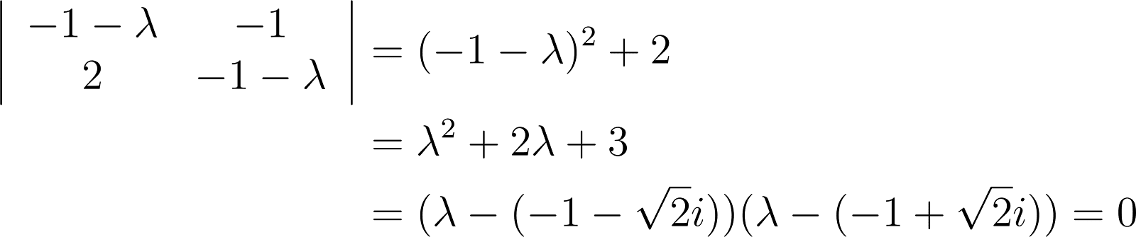
Chapter 7: Problem 16 Elementary Differential Equations and Boundary Value Problems 11
In each of Problems 16 and 17, solve the given system of equations by the method of Problem 13 of Section 7.5. Assume that t > 0.tx_ = _1 1 2 1 _ x 1
Read more -
Chapter 7: Problem 17 Elementary Differential Equations and Boundary Value Problems 11
In each of Problems 16 and 17, solve the given system of equations by the method of Problem 13 of Section 7.5. Assume that t > 0.tx_ = _2 5 1 2 _ x 1
Read more -
Chapter 7: Problem 18 Elementary Differential Equations and Boundary Value Problems 11
In each of Problems 18 and 19: a. Find the eigenvalues of the given system. G b. Choose an initial point (other than the origin) and draw the corresponding trajectory in the x1x2-plane. Also draw the trajectories in the x1x3- and x2x3-planes. G c. For the initial point in part b, draw the corresponding trajectory in x1x2x3-space.x_ = 1 4 1 0 1 1 4 0 0 0 1 4 x 1
Read more -
Chapter 7: Problem 19 Elementary Differential Equations and Boundary Value Problems 11
In each of Problems 18 and 19: a. Find the eigenvalues of the given system. G b. Choose an initial point (other than the origin) and draw the corresponding trajectory in the x1x2-plane. Also draw the trajectories in the x1x3- and x2x3-planes. G c. For the initial point in part b, draw the corresponding trajectory in x1x2x3-space.x_ = 1 4 1 0 1 1 4 0 0 0 1 10 x 2
Read more -
Chapter 7: Problem 20 Elementary Differential Equations and Boundary Value Problems 11
Consider the electric circuit shown in Figure 7.6.6. Suppose that R1 = R2 = 4 , C = 1 2 F, and L = 8 H. a. Show that this circuit is described by the system of differential equations d dt _I V _ = 1 2 1 8 2 12 _I V _, (32) where I is the current through the inductor and V is the voltage drop across the capacitor. Hint: See Problem 18 of Section 7.1. b. Find the general solution of equations (32) in terms of realvalued functions. c. Find I (t) and V(t) if I (0) = 2 A and V(0) = 3 V. d. Determine the limiting values of I (t) and V(t) as t . Do these limiting values depend on the initial conditions? R1 R2 L C FIGURE 7.6.6 The circuit in Problem 20. 2
Read more -
Chapter 7: Problem 21 Elementary Differential Equations and Boundary Value Problems 11
The electric circuit shown in Figure 7.6.7 is described by the system of differential equations d dt _I V _ = 0 1L 1C 1 RC _I V _, (33) where I is the current through the inductor and V is the voltage drop across the capacitor. These differential equations were derived in Problem 16 of Section 7.1. a. Show that the eigenvalues of the coefficient matrix are real and different if L > 4R2C; show that they are complex conjugates if L < 4R2C. b. Suppose that R = 1 , C = 12 F, and L = 1 H. Find the general solution of the system (33) in this case. c. Find I (t) and V(t) if I (0) = 2 A and V(0) = 1 V. d. For the circuit of part b, determine the limiting values of I (t) and V(t) as t . Do these limiting values depend on the initial conditions? C L R FIGURE 7.6.7 The circuit in Problem 21. 2
Read more -
Chapter 7: Problem 22 Elementary Differential Equations and Boundary Value Problems 11
In this problem we indicate how to show that u(t) and v(t), as given by equations (17), are linearly independent. Let r1 = + i and r1 = i be a pair of conjugate eigenvalues of the coefficient matrix A of equation (1); let (1) = a + ib and (1) = a ib be the corresponding eigenvectors. Recall that it was stated in Section 7.3 that two different eigenvalues have linearly independent eigenvectors, so if r1 _= r1, then (1) and (1) are linearly independent. a. First we show that a and b are linearly independent. Consider the equation c1a+c2b = 0. Express a and b in terms of (1) and (1) , and then show that (c1 ic2) (1) + (c1 + ic2) (1) = 0. b. Show that c1ic2 = 0 and c1+ic2 = 0 and then that c1 = 0 and c2 = 0. Consequently, a and b are linearly independent. c. To show that u(t) and v(t) are linearly independent, consider the equation c1u(t0)+c2v(t0) = 0, where t0 is an arbitrary point. Rewrite this equation in terms of a and b, and then proceed as in part b to show that c1 = 0 and c2 = 0. Hence u(t) and v(t) are linearly independent at the arbitrary point t0. Therefore, they are linearly independent at every point and on every interval. 2
Read more -
Chapter 7: Problem 23 Elementary Differential Equations and Boundary Value Problems 11
A mass m on a spring with constant k satisfies the differential equation (see Section 3.7) mu__ + ku = 0, where u(t) is the displacement at time t of the mass from its equilibrium position. a. Let x1 = u, x2 = u_, and show that the resulting system is x _ = 0 1 k m 0 _ x. b. Find the eigenvalues of the matrix for the system in part a. c. Sketch several trajectories of the system. Choose one of your trajectories, and sketch the corresponding graphs of x1 versus t and x2 versus t. Sketch both graphs on one set of axes. d. What is the relation between the eigenvalues of the coefficient matrix and the natural frequency of the spring-mass system? 2
Read more -
Chapter 7: Problem 24 Elementary Differential Equations and Boundary Value Problems 11
Consider the two-mass, three-spring system of Example 3 in the text. Instead of converting the problem into a system of four first-order equations, we indicate here how to proceed directly from equations (22). a. Show that equations (22) can be written in the form x __ = 2 3 2 4 3 3 x = Ax. (34) b. Assume that x = ert and show that (A r2I) = 0. Note that r2 (rather than r) is an eigenvalue of A corresponding to an eigenvector . c. Find the eigenvalues and eigenvectors of A. d. Write down expressions for x1 and x2. There should be four arbitrary constants in these expressions. e. By differentiating the results from part d, write down expressions for x_ 1 and x_ 2. Your results from parts d and e should agree with equation (31) in the text. 2
Read more -
Chapter 7: Problem 25 Elementary Differential Equations and Boundary Value Problems 11
Consider the two-mass, three-spring system whose equations of motion are equations (22). Let m1 = 1, m2 = 4/3, k1 = 1, k2 = 3, and k3 = 4/3. a. As in Example 3, convert the system to four first-order equations of the form y_ = Ay. Determine the coefficient matrix A. b. Find the eigenvalues and eigenvectors of A. c. Write down the general solution of the system. G d. Describe the fundamental modes of vibration. For each fundamental mode, draw graphs of y1 versus t and y2 versus t. Also draw the corresponding trajectories in the y1 y3- and y2 y4- planes. G e. Consider the initial conditions y(0) = (2, 1, 0, 0)T . Evaluate the arbitrary constants in the general solution in part c. What is the period of the motion in this case? Plot graphs of y1 versus t and y2 versus t. Also plot the corresponding trajectories in the y1 y3- and y2 y4-planes. Be sure you understand how the trajectories are traversed for a full period. G f. Consider other initial conditions of your own choice, and plot graphs similar to those requested in part e.
Read more